Introduction

1. Input Data

Input data for the main routines are astropy tables (see Data Tables), which provide all the functionality to manipulate tabular data, and to read/write in a variety of formats (ASCII, VOTable, FITS tables, etc.)

These input tables should have columns for at least angular coordinates and weights, but note the default names of columns can be overridden so there is no need to rename your original table (e.g. that infamous “RAJ_2000” instead of “ra”). Extra columns are welcome though as the name implies, are indeed extra and consume extra memory

Default name	Description
ra,dec	Right ascension and declination [deg]
z	Redshift (not needed in angular correlations)
wei	Weight of source
dcom	Comoving distance. Only used if calcdist=False

For example, data in FITS format can be read simply by

from astropy.table import Table
gals = Table.read('redgals.fits')  # read data
# If gals does not have a column for weights, just create one filled with 1's
gals['wei'] = 1.0

2. Set Up Input Parameters

Since there are quite a few parameters to deal, Gundam employs a special dictionary (see Munch) to pack and pass all of them at once. This dictionary also has attribute-like access with dot notation, meaning to access parameters you just type par.omegam (print matter density), par.h0=100. (set Hubble constant), etc. If you are used to ipython+tab completion you will certainly love this.

While you can create an input parameter dictionary from scratch, it is far easier to use gundam.packpars() to create a skeleton with default values, and then customize it to your needs. For example

import gundam as gun
par = gun.packpars(kind='pcf')    # Get defaults for a proj. corr. function
par.h0    = 69.5      # Change H0 [km/s/Mpc]
par.nsepp = 24        # Set 24 bins in projected separation [Mpc]
par.dsepp = 0.1       # Each of size 0.1 dex
par.estimator = 'LS'  # Pick Landy-Szalay estimator

# Can also specify values while creating the par object
par2 = gun.packpars(kind='acf', outfn='/test/angularcf')

# Quickly check all parameters by printing a nicely formated list
par2.qprint()

3. Get Counts & Correlations

Having read your data (gals and rans) and set up input parameters par, getting a projected correlation function is as easy as

cnt = gun.pcf(gals, rans, par, nthreads=1)

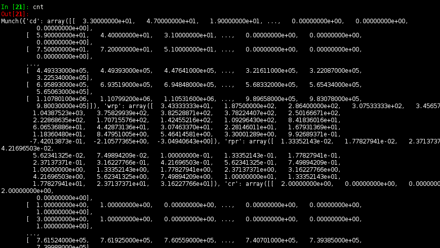
The output object cnt is, again, a Munch dictionary that holds the correlation function cnt.wrp, the projected bins mid-point cnt.rpm, and many others. Here we show that the data and random samples had ~84k and 400k galaxies, respectively.

cnt.qprint()

# =================  Projected Correlation  =================
# Description :: Full projected autocorrelation
# npt         :: 84383
# npt1        :: 400000
# rpl         :: [ 0.1 ... 1.58113882522 ... 16.8522765348 ]
# rpm         :: [ 0.124173954464 ... 1.96336260485 ... 20.9261381905 ]
# rpr         :: [ 0.148347908929 ... 2.34558638447 ... 24.9999998462 ]
# wrp         :: [ 214.431631437 ... 22.5684208374 ... 4.51112595359 ]
# wrperr      :: [ 20.4245915831 ... 1.15641601016 ... 0.435505255 ]
# dd          :: [ 2082.0 ... 84.0 ... 26.0 ]
#                [ ...  ... ]
#                [ 1428490.29 ... 1136520.2 ... 823343.33 ]
# rr          :: [ 1084.0 ... 918.0 ... 749.0 ]
#                [ ...  ... ]
#                [ 26894309.95 ... 22249661.39 ... 17933389.42 ]
# ......

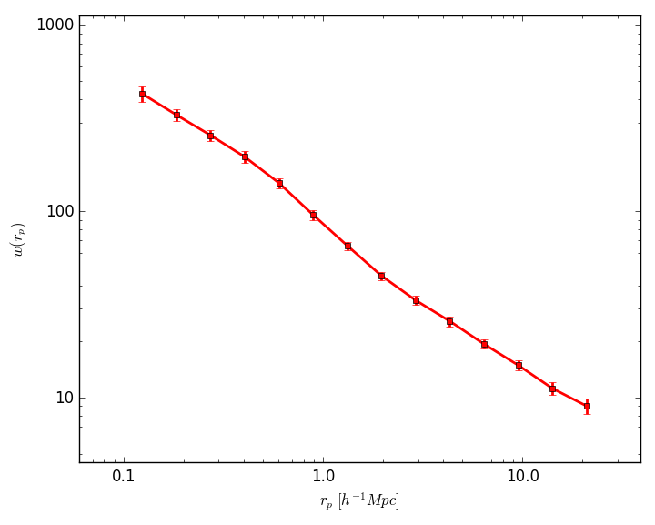
A plot is worth a thousand words, so let’s do a good graphic of \(w(r_p)\) by typing gun.cntplot(cnt, factor=2.) (the 2x factor is due to xxxx)

4. Going Parallel

To speed things up, Gundam can count pairs in parallel using multiple cores. Just set nthreads as in

cnt = gun.pcf(gals, rans, par, nthreads=8)

That’s all. Under the hood, the software divides the counting process in several declinations stripes, computes the pairs in each, and adds everything up at the end. OpenMP threads are created and scheduled by the underlying Fortran code.

5. Typical Use Cases

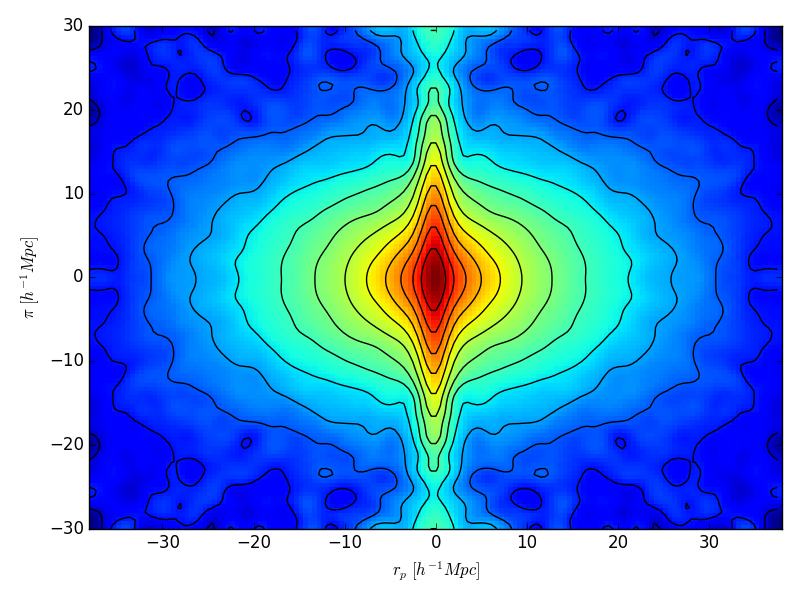
Check God’s Fingers

Gundam can calculate and plot 2D correlation functions in a few lines. Let’s see a self-explanatory example for 100k luminous red galaxies from SDSS DR7 (included in /examples directory)

from astropy.table import Table
import gundam as gun

# READ DATA
gals = Table.read('./examples/DR7-lrg.fits')
rans = Table.read('./examples/DR7-lrg-rand.fits')
gals['wei'] = 1.0
rans['wei'] = 1.0

# DEFINE INPUT PARAMETERS
par = gun.packpars(kind='pcf')
par.outfn     = './examples/LRGs'  # Base name of output files
par.estimator = 'LS'    # Choose Landy-Szalay estimator
par.nsepp     = 76      # Number of bins in projected separation rp
par.seppmin   = 0.01    # Minimum rp [Mpc/h]
par.dsepp     = 0.5     # Bin size in rp [Mpc/h]
par.logsepp   = False   # Use linear spaced bins
par.nsepv     = 60      # Number of bins in radial separation pi
par.dsepv     = 0.5     # Bin size in pi [Mpc/h]

# GET PCF
cnt = gun.pcf(gals, rans, par)

# PLOT A SMOOTHED 2D PCF
gun.cntplot2D(cnt, slevel=8)

which produces this cool figure. Anything familiar? Perhaps the Fingers of God? Kaiser squashing?

Lessons on Integration

So far so good, but how do you set the radial integration limit of w(rp)? There are two ways:

• The long way : you set radial bins (nsepv, dsepv) accordingly. For example, to integrate up to 40 Mpc make 40 bins of 1 Mpc with nsepv=40, dsepv=1.0
• The short way : you set radial bins (nsepv, dsepv) accordingly. For example, to integrate up to 40 Mpc make 1 bin of 40 Mpc with nsepv=1, dsepv=40.

No need to point out that the short way is faster. Hence, if you don’t mind about intermediate bins just go straight with a single “fat” bin.

Note, however, that if you request a set of radial bins, i.e. nsepv>1, the code will: (1) calculate projected correlation function at each radial bin, and (2) sum each contribution. This can be different from adding the counts from all radial bins and then applying the estimator because empty bins are not necessarily the same in the DD, RR and DR terms. A single fat bin will have higher signal and less noise, especially at small separations.

Printing Nicely

While the dictionaries that store counts and/or parameters are useful objects, they do not print nicely due to amount and dimensions of the various arrays inside. Again, there are two ways to go around:

• Use gun.qprint() method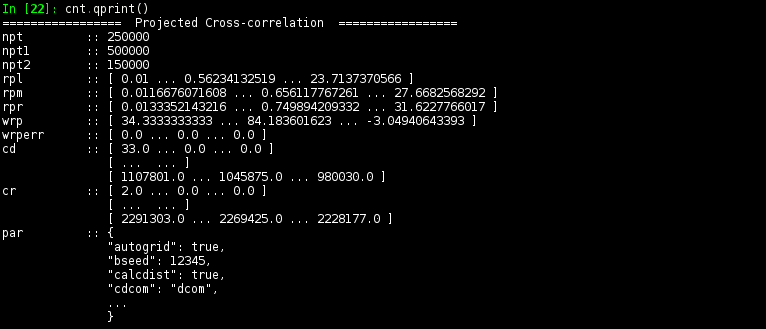

  

• Use gun.cnttable() routine to pop up a table of counts in your browser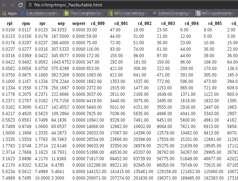

  

Or you can always try your luck using (i)python regular print

Further Examples

Data and code for 3 examples of using Gundam are provide in the repo (example_lrg.py, example_pcf.py and example_redblue.py).

6. Coordinates & Distances

The radial, projected and redshift-space distance between two galaxies i and j are calculated as

\(\pi = |dc_i-dc_j|\)

\(r_{p}^{2} = 4 dc_i dc_j [(x_i-x_j)^2 + (y_i-y_j)^2 + (z_i-z_j)^2]\)

\(s^2 = \pi^2 + r_{p}^{2}\)

where dc is the comoving distance in the chosen cosmology and (x, y, z) are the rectangular coordinates given by

\(x = 0.5 \cos(dec)\sin(ra)\)

\(y = 0.5 \cos(dec)\cos(ra)\)

\(z = 0.5 \sin(dec)\)

By default the comoving distances are calculated with astropy’s cosmology module using a FLRW cosmology with a cosmological constant and curvature (LambdaCDM). If you prefer another, just modify the corresponding code in the main Gundam routines, or even better, append your own distances to the input tables and set calcdist=False

7. Routines, Cells & Counts

All Fortran routines are stored in the cflibfor library, under the module called mod. Feel free to directly use these, for example

import cfibfor as cff
cff.mod.bootstrap(10,4,124567)

or through Gundam

import gundam as gun
gun.cff.mod.bootstrap(10,4,124567)

Of course the number of cells to use (i.e. mxh1, mxh2, mxh3) has some impact in the performance and the optimum values depends on the sample characteristics, the binning adopted and even the hardware employed. Gundam will try to guess values for these parameters based on simple fittings to galaxy data extracted from the Millennium Simulation. They should work well as starting values for many use cases but depending your needs, you might want to fine tune these. Just remember to keep it reasonable. For example, if you have half million objects, setting mxh1=4 or mxh1=400 is not wise in most cases. Expect typical variations of 3-30% in performance for a range of reasonable values.

Note the counting routines actually return half of real pairs, so depending the case you might want to multiply by 2. The estimators for all implemented correlation functions already do this for you.