Pixel Ordering Methods

To increase the performance of linked list algorithms, spatial data is divided in “pixels” and these pixels are sorted by different methods. The rows of the input data table can be rearranged according to this pixel index, so that nearby structure in real space are also close in computer memory space. Once input data is sorted, traversing the linked list will generate many more cache hits.

This is quite similar to Morton-curve or Hilbert-curve techniques used in computer science to map multidimensional data into a one dimensional index.

Note these “pixels” have nothing to do with the cells used by the linked list algorithm. The parameter pxorder controls the method to sort the pixels. Available options are:

• ‘natural’
  Pixels are sorted in lexical order by three keys, Z-DEC-RA, in that order. This is usually the fastest option as it more closely matches the mechanics of the counting algorithm. The number of pixels are set to (mxh3,mxh1,mxh2)
• ‘morton_dir’
  2D Morton-curve ordering using the RA-DEC values directly, i.e. no division in pixels
• ‘morton2’
  Pixels are sorted by 2D Morton-curve in RA-DEC
• ‘morton3’
  Pixels are sorted by 3D Morton-curve in RA-DEC-Z
• ‘hilbert2’
  Pixels are sorted by 2D Hilbert-curve in RA-DEC
• ‘hilbert3’
  Pixels are sorted by 3D Hilbert-curve in RA-DEC-Z

Note these are experimental features mainly for testing purposes. You do not need to fuss with these options unless you are looking for fun. Plus, in most cases the default natural order is the fastest option.

The following images illustrate how pixel sorting rearranges a list of ra-dec coordinates into nearby patches. The vertical axis is the index of the ra-dec point in the list (in log scale for clarity).

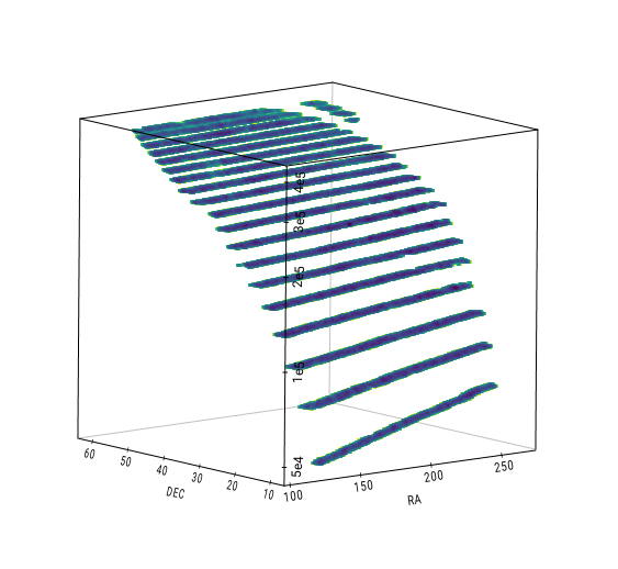
Natural pixel ordering

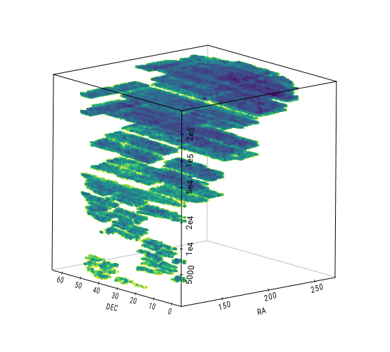
Morton pixel ordering

Custom RA Boundaries

The area in the sky occupied by a sample or survey can be composed of multiple scattered “patches” at both sides of the RA=0 limit. In order to efficiently grid and sort such a sample, the area enclosing all of its objects should be minimal, which can be difficult to find out automatically.

For example, if a survey is composed of two equatorial 1 deg^2 patches, one beginning at RA=355 deg and the other beginning at RA=5 deg, the grid can extend from 5 to 356 deg or, more conveniently, from 355 to 6 deg. The input parameter custRAbound can be set to indicate such limits. In this case, setting custRAbound = [355., 6.] will create a much smaller grid and routines will perform faster.

Gundam will try to guess if a sample crosses the RA=0 limit (see gundam.cross0guess()).